Licensed under the CC BY-NC-SA
Abstract
In this work of the methodological direction, a new approach to the calculation of thermodynamic characteristics of chemical processes of reduction of metal ores is proposed. The possibility of constructing interpolation equations of regression of temperature dependencies of isobaric-isothermal potential due to the course of a chemical reaction (Gibbs energy) is considered. Also – the dependence of the Gibbs energy on the oxidation state of the metal in the ore mixture during reduction in metallurgical furnaces. A new differential form of expression of a chemical reaction has been proposed, which shows the qualitative dynamics of redox processes, in contrast to the quantitative one, which is engaged in chemical kinetics. The developed methodology will be able to help in the creation of software in the automation of metallurgical processes, especially in the field of “green technologies”, i.e., solid-phase reduction of ore materials with carbon-free reducing agents (hydrogen, ammonia, etc.).
Keywords: chemical thermodynamics, redox reactions, Gibbs energy, metallurgy, green technologies, hydrogen recovery, regression equation, metrology of calculations
Introduction
If the beginning of the 2000s could be called the “Information Technology” era, then the 20-ies of the 21st century, they mark the beginning of a new era – “Green technologies” [1], for the purpose of preserving the environment, preserving climate on Earth, preserving humanity. It is in these spheres of scientific developments in the coming years that the main funds of states and business will be poured in the coming years. Decarbonization, struggle for reducing greenhouse gas emissions, reducing the impact of the economy on the climate are probably the main trends of today [2].
But not only in the field of energy requires changes with the “Green Deal” and the rejection of carbonic raw materials. It is also important for all chemical and metallurgical technologies that use coal, petroleum products and natural gas and their derivatives containing carbon.
To obtain metals from ore raw materials, carbon C, CH4 methane, CO+H2 converter gas is now mainly used as a reducing agent [3]. As a result, significant amounts of carbon dioxide CO2 are thrown into the atmosphere.
An important task of future metallurgy is to introduce alternative methods of recovery of metallic ores, such as “green” hydrogen H2 (that is, not obtained by steam conversion of coke or methane) [4]. Also, complete automation of processes using computer programs.
But this requires some rethinking of the energy of the chemical oxidative reactions with the participation of compounds that are part of metal ores.
Calculation and modeling techniques
For the calculation of values of free energy Gibbs [5,6] (at certain temperatures) for chemical reactions the formation of iron oxides and their reactions of their restoration of hydrogen were used tables of thermodynamic values [6,7]. To calculate the Gibbs free energy values (at certain temperatures and states of iron oxidation), according to the calculated regression equations, the capabilities of the WolframAlpha program were used [8]. Also, a number of graphs were built with this program. Gnuplot5 was used to build 3D-graphs of Gibbs energy and equilibrium hydrogen pressure from the degree of oxidation of the ore mixture and temperature [9]. To obtain regression equations based on the calculated tabular values of Gibbs energy at different temperatures, the Mathcad program was used [10]. Also, most of the graphs were created. IrfanWiev was used to create and photograph files in the JPG format [11].
Investigation of cross-interpolation of regression equations in Fe - O
We are all used to the classical (stichiometric) appearance of the equation of chemical reaction, where one (two, three) molecules (atoms) of the source reagents react and - through the sign of equation we get one (two, three) molecules (atoms) of reaction products [12]. And then, suddenly we move to the masses of substances in g-moles that have reacted and the masses of substances in the formed moles. But, in 1 g-mole of substance are not one (two, three) molecules (atom), and, according to the Number of Avogadro – 6.022*1024 molecules (atoms) [13]. This number, according to the laws of chemical kinetics, cannot react at the same time. 1 g of solid or liquid substance has a volume of several tens of cubic centimeters, and gaseous – 22.41 liters [13]. And here they already come to the fore not only the number of reagents, but also the speed of diffusion of reacting molecules. In addition, the reaction products formed on the surface of the reagent particles can interfere with the diffusion of subsequent molecules deep into the particles. This was pointed out by J.Gibbs when introducing the concept of chemical potential in heterogeneous processes [5]. Thus, the reagent particle turns into a multilayered “pie” with a certain gradient of transitional concentrations of the output reagents and reaction products. And then the sign of the equation in the classical form of a chemical reaction, which looks like an instant transformation of reagents into reaction products, does not correspond to the real quantitative and qualitative course of the reaction. Chemical kinetics in this case shows only the quantitative indicator of the process [13]. Qualitative classic methods are not shown.
With regard to real materials, such as natural ore concentrates, the picture is even more confusing, because they may have a whole set of different compounds of ore metal with different valences. For example, iron ores may have joints of trivalent and divalent iron (hematite, magnetite, iron carbonate, pyrite, etc.) [5]. During heating in the furnaces and the restoration of iron, various transitional forms between hematite, magnetite, wüstite and metallic iron in different proportions during recovery are formed.
If you imagine the process of reacting 1 mole of reagent containing 6.022*1024 molecules, it will be average, as close as possible to the normal distribution of Gauss [14], the process of changing the degree of oxidation (when the oxide is formed) or restoration (reduction of iron oxidation when recovering metal).
To develop a single model of the reduction process, it is necessary that all these transitional forms with different degrees of iron oxidation are expressed in a single form. But in the literature sources, the form of expression of oxides in the form of FexOy usually prevails [13], and for wüstite, either the form FenO (where n is close to 0.947) or FeOn (where n is close to 1.056) is used [5,7].
In this expression, each reaction has a different number of oxide atoms entering into the reaction and therefore thermodynamic quantities cannot be compared without transition coefficients. Therefore, this does not make it possible to programmatically combine the processes of transformation of transitional forms of oxidation or metal reduction.
It is possible to bring all oxidized forms of the metal to the same denominator by expressing the formula of the oxide in the form of Fe1-mOm, where m is the oxidation state of the metal as the fraction of oxygen in the molecule reduced to one. That is, in the classic FexOy formula:
m = y/(x + y) (1)
Thus, we obtain for the wüstite m = 0.51361; for magnetite m = 0.57143; for hematite m = 0.6. And for pure metal Fe: m = 0.
In this form, the oxide, regardless of its oxidation level, always participates in reactions only in the amount of 1 g-mol, and the general reaction for the formation of iron oxides will look like this:
(1-m) Fe + 0.5m O2 = Fe1-mOm (2)
Since the tabular data of enthalpy and entropy at different temperatures to calculate the Gibbs free energy of the formation of iron oxides ∆ƒGoT [2,7] are given in the literature for the reactions presented in the classical form of FexOy, in order to convert them to the form Fe1-mOm, it is necessary to divide the calculated equations for ∆ƒGoT[FexOy] by the number of atoms in the corresponding oxide molecule. For wüstite Fe0.947O, we divide the calculated Gibbs energy by 1.947, for magnetite Fe3O4 by 7, and for hematite Fe2O3 by 5. After that, we calculate the equation of regression of the temperature dependence of the Gibbs energy on the formation of iron oxides. And thus, we get three equations in the form ∆ƒGo[Fe1-mОm].
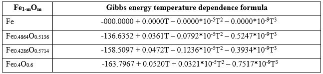
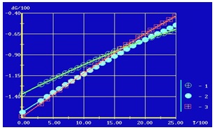
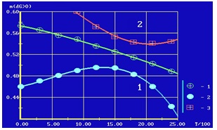
According to the tabular data [2,7], we calculate the value of Gibbs free energy at different temperatures in the range T = 0 ÷ 2500°K for the metal oxidation reaction per one oxide molecule. The temperature range of calculations was deduced to 0°K in order for the obtained regression equations to be universal, suitable for all subsequent reactions involving metal oxides with other reagents, for example, reducing agents. In the region between 1600 ÷ 1700°K for iron oxides, the transition of the solid phase to the liquid phase occurs with a certain temperature effect. Based on the data obtained, we plot ∆ƒGo[Fe1-mOm] = ƒ(T) for wüstite, magnetite and hematite (Fig. 1) and calculate the corresponding third-order regression equations of the type ∆ƒGo = A + BT + CT2 + DT3 (Tab. 1), as well as the values of the coefficients A, B, C, D for the equations of the formation of wüstite, magnetite and hematite (Tab. 2).
For an unoxidized metal, the Gibbs energy of oxide formation is zero, so all coefficients of a 3rd-order polynomial for the metal are also zero.
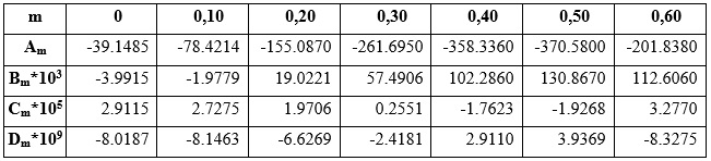
Table 1. Formulas for Gibbs energy temperature dependence regression equations for Metal, Wüstite, Magnetite and Hematite
Table 2. Values of the coefficients of the equations for the formation of iron oxides
Figure 1. Temperature dependence of Gibbs energy in the formation of iron oxides
1 – wüstite; 2 – magnetite; 3 - hematite
If you place on the graph the change in the value of the coefficients of the regression equation A, B, C, D according to Table 2 of values mi then you can calculate the regression equation in the range m = 0 ÷ 0.6, which will show the value of the average value of each of the coefficients that will be in each moment of reaction is somewhere between these points according to the interpolation second theorem of Bolzano-Koshi (the theorem on the intermediate value of continuous function), which states that if a continuous function takes two values “a” and “b”, it will also accept the value of “c” on the segment between them [16].
In the case of the renewable process, the value of the coefficients A, B, C, D will gradually pronounced from their value at m = 0.6 to m = 0.5136. And then – to m = 0 with the complete restoration of the metal.
In order to carry out cross-interpolation between the Gibs energy temperature equations, there are four graphs on which the abscissa will be m, and on the ordinate axis-the magnitude of the i-th value of the corresponding coefficient of the Gibs energy dependence equation.
Further, we carry out a regression analysis to build an interpolation curve between all points on the axis of values m according to Table. 2. As a result, we get four regression equations in the form of complex polynomials. In this case, the order of polynomials should be limited to the accuracy of calculations of coefficients A, B, C, D = ƒ(m) is sufficient and to minimize possible oscillations of curves [17,18], especially in a large gap between mo = 0 and m1 = 0.5136 .
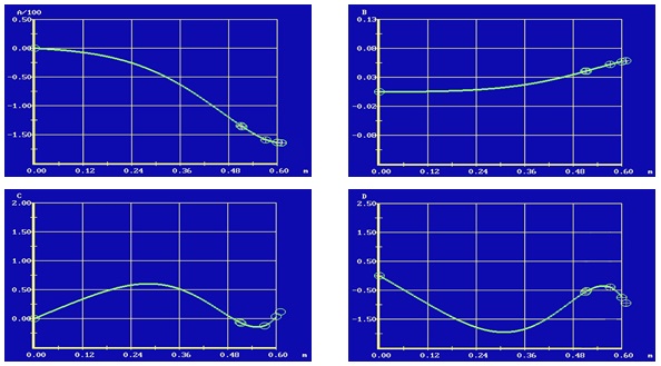
As a result, we get four graphs of cross-interpolation of the Gibs energy dependence equations for the formation of iron oxides of any composition ∆ƒGo[Fe1-mОm] with variable value m. The graphs of these equations are presented in Fig. 2–4.
Rice. 2–4. The size of coefficients A, B, C, D in the equation of cross-interpolation depending on the level of oxidation of iron
The general equation for the Gibbs energy temperature dependence ∆Go[Fe1-mОm] will look like this:
∆ƒGo[Fe1-mОm] = Am + BmT + CmT2 + DmT3 (3)
where: Am, Bm, Cm, Dm are the polynomials of the coefficients in the form of functions ƒ(m).
Based on these data, we calculate the regression equations of cross-interpolation for the coefficients of temperature dependence ∆ƒGo[Fe1-mOm] within m = 0 ÷ 0.6 and T = 0 ÷ 2500°K.
Am = -39.1485m – 122.0880m2 – 419.9718m3 – 1229.8400m4 + 313.5867m5 + 1345.0990m6 + 2376.4400m7 (4)
Bm = (-3.9915m – 32.6460m2 + 252.3352m3 + 280.2343m4 + 346.7170m5 – 757.5040m6 – 584.8810m7)*10-3 (5)
Cm = (2.9115m – 0.7663m2 + 3.3180m3 – 31.9305m4 – 32.5412m5 + 17.6554m6 + 131.6203m7)*10-5 (6)
Dm = (-8.0187m – 1.5452m2 – 5.5484m3 + 75.8750m4 + 98.4471m5 – 46.4668m6 – 339.1803m7)*10-9 (7)
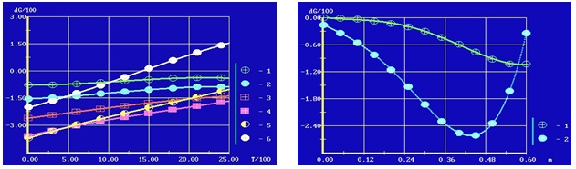
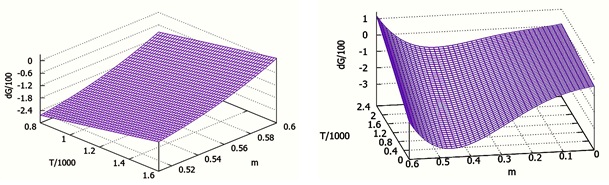
According to the obtained equations, we calculate the value of the Gibbs free energy of iron oxidation ∆ƒGo = Am + BmT + CmT2 + DmT3 in the range m = 0 ÷ 0.6 (Fig. 5). Based on the equations obtained in (4-7), we calculate a series of regression equations for the dependence of ∆ƒGo, kJ/mol on m and T, the graphs of which are presented in Fig.5-9.
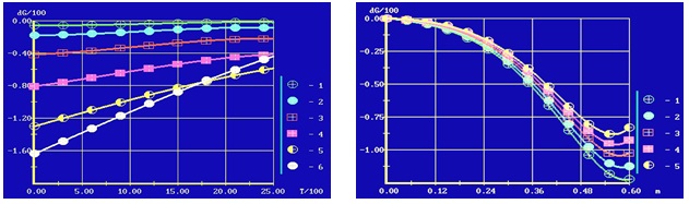
Figure 5. Temperature dependence of ∆ƒGo on the oxidation state of iron m.
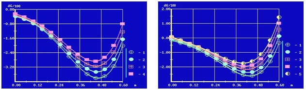
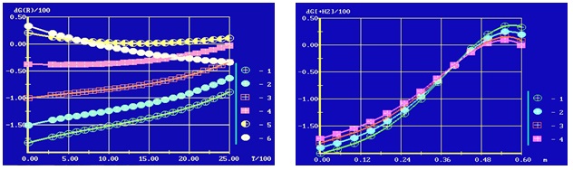
Figure 6. Dependence of ∆ƒGoT on the oxidation state of iron in the range m = 0 ÷ 0.6 and temperatures in the range T = 800 ÷ 1600°K.
1 – (m = 0.1); 2 – (m = 0.2); 3 – (m = 0.3); 1 – 800оК; 2 – 1000оК; 3 – 1200оК;
4 – (m = 0.4); 5 – (m = 0.5); 6 – (m = 0.6) 4 – 1400оК; 5 – 1600оК
Figure 7. Reservoir of energy ∆ƒGoT leads the oxidation stage of the diapason m = 0.5 ÷ 0.6 and temperatures in the diapason T = 800 ÷ 1600°K
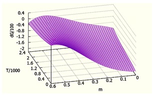
Figure 8. 3D-graph of the energy residue of the Gibbs energy ∆ƒGo leading the oxidation stage of the diapason m = 0.5 ÷ 0.6 and the temperature in the diapason T = 800 ÷ 1600°K
1 – 800оК; 2 – 1000 оК; 3 – 1200 оК;
4 – 1400 оК; 5 – 1600 оК
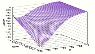
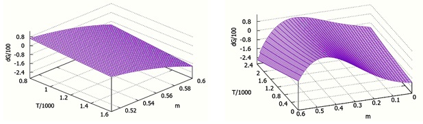
Figure 9. 3D-graph of the dependence of Gibbs energy ∆ƒGo on the oxidation state of iron in the range m = 0 ÷ 0.6 and temperatures in the range T = 0 ÷ 2400°K
From Fig. 7 shows that in the range m = 0.5 ÷ 0.6, minima of Gibbs energy values are observed at certain values of the oxidation state of iron. That is, at these points, at certain temperatures, the oxide system is as stable as possible. And the higher the temperature, the greater the peak of stability shifts towards a lower degree of iron oxidation – if at 800°K this zone of maximum stability is close to almost pure hematite, then at 1400°K the zone of stability shifts to magnetite.
Differential equation of metal oxidation
Suppose that a metal, or the sum of its oxides with a certain level of oxidation, reacts with another portion of oxygen ∆m*[0.5O2], then the total reaction will look like:
((1-m) - ∆m) Fe1-mOm + ∆m [0.5 O2] = (1-m) Fe1-m-∆mOm+∆m (8)
If the amount of oxygen entering into the reaction is reduced to almost zero (one atom), then the equation can be written in differential form:
((1-m) - ∆m) Fe1-mOm + dm [0.5 O2] = (1-m) Fe1-m-dmOm+dm (9)
Let's reduce the reaction to one oxygen atom by dividing the equation by dm:
((1-m) - ∆m)/dm Fe1-mOm + 0.5 O2 = (1-m)/dm Fe1-m-dmOm+dm (10)
Let's divide the numerator on the left side of the equation into two parts:
(1-m)/dm Fe1-mOm – Fe1-mOm + 0.5 O2 = (1–m)/dm Fe1-m-dmOm+dm (11)
Let's transfer the differential term of the reaction from the right side of the equation to the left, and Fe1-mOm (as a constant) to the right side and represent the final sum of oxides and the initial one in the form of a differential difference. As a result, we get a reaction of oxide formation with a certain degree of oxidation in differential form:
–(1-m) [Fe-dmOdm]/dm + 0.5 O2 = Fe1-mOm (12)
According to this reaction, the Gibbs energy is also differentiated:
∆ƒGoT[D] = ∆ƒGoT + (1–m)*dƒGoT/dm (13)
In the future, the classical process of direct oxidation (reduction) will be denoted by the index [R], and gradual additional oxidation (deoxidation) in differential form by the index [D].
If the expression obtained in equation (11) is solved with respect to changes in the amount of oxygen and written in the form:
then we can see that it is analogous to the Lagrange formula for a continuous function [18].
The expression in equation (13) could be compared with the expression for the chemical potential [5] (for this reaction – oxygen):
But the difference is that in this case, the temperature and mole fractions of the other components are variable, and the variable magnitude m does not represent the number of molecules nO2, but the molecular fraction of one.
The regression equation for the coefficients Am, Bm, Cm, Dm in the equation ∆ƒGo[Fe1-mOm] = ƒ(T) can be differentiated, then:
∆ƒGo[D] = (Am+(1–m)(dAm/dm)) + (Bm+(1–m)(dBm/dm))T + (Cm+(1–m)(dCm/dm))T2 + (Dm+(1–m)(dDm/dm))T3 (16)
Based on (16), we calculate the derivatives of the coefficients of temperature dependence ∆ƒGo′ within m = 0 ÷ 0.6 and T = 0 ÷ 2500oK:
(A)′ = -39.14847 – 244.1760m – 1259.9154m2 – 4919.3600m3 + 1567.9335m4 + 8070.5940m5 + 16635.0800m6 (17)
(B)′ = (-3.9914 – 65.2920m + 757.0056m2 + 1120.9372m3 + 1733.5850m4– 4545.0240m5–4094.1670m6)*10-3 (18)
(C)′ = (2.9115 – 1.5327m + 9.9539m2 – 127.7220m3 – 162.7058m4 + 105.9322m5 + 921.3421m6)*10-5 (19)
(D)′ = (-8.0187 – 3.0904m – 16.6452m2 + 303.5000m3 + 492.2357m4 – 278.8005m5 – 2374.2621m6)*10-9 (20)
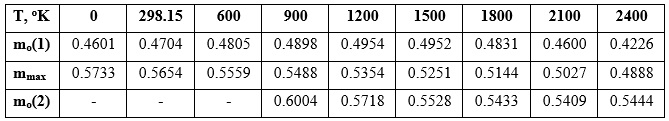
We multiply them by (1-m). According to the obtained equations, we calculate the coefficients for ∆ƒGo[D] = Am[dm] + Bm[dm]T + Cm[dm]T2 + Dm[dm]T3 in the range m = 0 ÷ 0.6 with the desired step m, for example – 0.1 (Table 3).
Table 3. The value of the coefficients of the differential equation of the temperature dependence of Gibbs energy as a function of m:
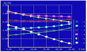
According to Table 3, the values of ∆ƒGo[D] depending on T and m, presented in Fig. 9 - 14.
Figure 9. Dependence of the Gibbs differential energy expression on m = 0 ÷ 0.6 in the range T = 0 ÷ 900°K
Figure 10. Dependence of the Gibbs differential energy expression on m = 0 ÷ 0.6 in the range T = 1200 ÷ 2400°K
1 – (Т = 0оК); 2 – (Т = 298.15оК); 1 – (Т = 1200оК); 2 – (Т = 1500оК); 3 – (Т = 1800оК);
3 – (Т = 600оК); 4 – (Т = 900оК); 4 – (Т = 2100оК); 5 – (Т = 2400оК);
Figure 11. Temperature dependence of the differential expression of Gibbs energy at different values of m.
Figure 12. Comparison of the Gibbs energy ∆ƒGoT[R] and its differential expression ∆ƒGoT[D] depending on the oxidation state m at T = 1200oK.
1 – (m = 0.1); 2 – (m = 0.2); 3 – (m = 0.3); 1 – ∆ƒGoT[R]; 2 – ∆ƒGoT[D]
4 – (m = 0.4); 5 – (m = 0.5); 6 – (m = 0.6)
Figure 13. 3D-graph of the dependence of Gibbs energy ∆ƒGo[D] on the oxidation state of iron in the range m = 0.5 ÷ 0.6 and temperatures in the range T = 800 ÷ 1600°K
Figure 14. 3D-graph of the dependence of Gibbs energy ∆ƒGo[D] on the oxidation state of iron in the range m = 0 ÷ 0.6 and temperatures in the range T = 0 ÷ 2400°K
Example for the magnetite to hematite oxidation reaction (∆m from m1 = 0.5714 to m2 = 0.6). Calculation of the coefficient A∆m in the polynomial of the Gibbs energy temperature regression equation
To begin with, let's calculate the Gibbs energy using the classical method [1,2,5,11,12]:
2 Fe3O4 + 0.5 O2 = 3 Fe2O3 (21)
∆ƒGo[R] = 3*∆GoT[Fe2O3] – 2*∆GoT[Fe3O4] (22)
∆ƒGo[R] = -237.8148 + 118.5554*10-3T + 2.2120*10-5T2 – 5.7673*10-9T3 (23)
In this function, we get the coefficient A∆m = -237.815.
In order to translate this equation into the form of representing oxides as Fe1-mOm, it is necessary to calculate the number of atoms in the molecules of hematite and magnetite by multiplying by the coefficients of the equation. For magnetite, the molecule of which consists of 7 atoms, it is 7x2 = 14, and for hematite it is 5x3 = 15. Then we can write the equation as:
14 Fe0.4286O0.5714 + 0.5 O2 = 15 Fe0.4O0.6 (24)
∆ƒGo[R] = 15*∆ƒGo[Fe0.4O0.6] – 14*∆ƒGo[Fe0.4286O0.5714] (25)
∆ƒGo[R] = -238.943 + 118.8928*10-3T + 2.1093*10-5T2 – 5.5091*10-9T3 (26)
In this function, we get the coefficient A∆m = -238.9430.
Now let's calculate the Gibbs energy using the differential equation:
for magnetite at m = 0.5714: Am = -158.5130 (according to equation (4)) ; then: (1 – m)dA/dm = -115.6790;
for hematite m = 0.6: Am = -163.8750; then: (1 – m)dA/dm = -37.9623.
A∆m = A[0.5714] + (1–m)(A[0.6] – A[0.5714])/∆m = -158.513 + 0.4286(-163.8750 – (-158.5130))/0.0286 (27)
In this case: 0.4286/0.0286 = 15, then:
A∆m = -158.5130 + 15*(-5.3620) = -158.5130 – 80.3550 = -238.8680 (28)
Integral method
A∆m = -158.5130 + 15*(-5.3628) = -158.5130 – 80.4426 = -238.9560 (30)
As you can see, the A∆m coefficient is calculated quite accurately. In the same way, other coefficients of the Gibbs energy temperature dependence equation can be calculated.
Reduction reactions of iron oxides with hydrogen in the range:
m = 0 ÷ 0.6; T = 0 ÷ 2500oK
As in the case of the reactions for the formation of metal oxides, when reducing it, we can consider the reduction reaction in the classical form, where the oxides and the reducing agent are on the left, and the end products immediately appear through the sign of the equation – metal and water vapor. But, as noted above, 6.022*1024 molecules of iron oxides with different valences cannot simultaneously react with hydrogen inside pieces of ore of a certain size. Therefore, the differential equation of the gradual process of reducing the level of oxidation of the metal from the initial average level of mo to m = 0, when all the ore is reduced to the metal, is more indicative. During this process, the amount of energy and hydrogen needed to complete the process will change. Let's first consider the classic direct recovery process.
The universal formula for the process of direct reduction of iron oxides will look like this:
1/m Fe1-mOm + H2 = (1–m)/m Fe + H2O (31)
The Gibbs energy for the direct reduction reaction (31) is as follows:
∆rGo[RH2] = ∆ƒGo[H2O] – 1/m ∆ƒGo[Fe1-mOm] (32)
To calculate ∆rGo[Fe1-mOm], the coefficients from the equation of cross-interpolation of iron oxide formation reactions can be used. Also, use the equation for the Gibbs energy of water formation in the range T = 0 ÷ 2500°K, calculated according to tables [2,7]:
∆ƒGo[H2O] = -239.8713 + 37.0829*10-3T + 1.2191*10-5T2 – 2.2955*10-9T3; (33)
Then:
∆rGo[RH2] = (A[H2O] – 1/m A[Fe1-mOm]) + (B[H2O] – 1/m B[Fe1-mOm])T + (C[H2O] – 1/m C[Fe1-mOm])T2 + (D[H2O] – 1/mD[Fe1-mOm])T3 (34)
Finally, we get the coefficients for deducting ∆rGo[RH2] depending on T and m:
AR = -200.7228 + 122.0880m + 419.9718m2 + 1229.8400m3 – 313.5867m4 – 1345.0990m5 – 2376.4400m6 (35)
BR = (41.0743 + 32.6460m – 252.3352m2 – 280.2343m3 – 346.7170m4 + 757.5040m5 + 584.8810m6)*10-3 (36)
CR = (-1.6924 + 0.7663m – 3.3180m2 + 31.9305m3 + 32.5412m4 – 17.6554m5 – 131.6203m6)*10-5 (37)
DR = (5.7232 + 1.5452m + 5.5484m2 – 75.8750m3 – 98.4471m4 + 46.4668m5 + 339.1803m6)*10-9 (38)
According to the resulting equations, we calculate the coefficients for ∆rGo[RH2] = AR + BRT + CRT2 + DRT3 in the range m = 0 ÷ 0.6. And then we calculate, according to the obtained coefficients, the values of ∆rGo[RH2] depending on T and m. Based on these data, we calculate a number of regression equations of the dependence ∆rGoT[RH2], kJ/mol depending on m and T. Graph of the temperature dependence of the Gibbs energy of direct reduction of iron by hydrogen ∆rGo[RH2] at different values of oxidation of the metal of the ore mixture is presented in Fig.15-18.
Figure 15. Temperature dependence of ∆rGo[RH2] at different oxidation values m
Figure 16. Dependence of ∆rGoT[RH2] on the oxidation state of the ore mixture at temperatures T = 0 ÷ 900°K
1 – (m = 0.1); 2 – (m = 0.2); 3 – (m = 0.3); 1 – (Т = 0оК); 2 – (Т = 298.15оК);
4 – (m = 0.4); 5 – (m = 0.5); 6 – (m = 0.6) 3 – (Т = 600оК); 4 – (Т = 900оК);
Figure 17. Dependency ∆rGoT[RH2] in the degree of acidification of the ore at temperatures T = 1200 ÷ 2400oK
Figure 18. 3D-graph dependency ∆rGo[RH2] in the degree of oxygenation of the ore m = 0 ÷ 0.6 and on the temperature T = 0 ÷ 2400oK
1 – (Т = 1200оК); 2 – (Т = 1500оК); 3 – (Т = 1800оК);
4 – (Т = 2100оК); 5 – (Т = 2400оК);
Based on the calculations presented by the graphs in Fig. 19-23, it can be seen that the curves of Gibbs energy values, depending on the level of oxidation of the ore mixture and temperature, have maxima going into the positive region, i.e., with such parameters, the free flow of reduction reactions is impossible. The parameters of these regions, in which ∆rGoT[RH2] > 0, as well as at which points the value of ∆rGoT[RH2] reaches its maximum, are presented in Table 4 and graphically in Fig.19.
Table 4. Parameters of the oxidation state m and temperature T°K, which delimit the zones of positive and negative values ∆rGoT[RH2]
Figure 19. The zones of demarcation of positive and negative values ∆rGoT[RH2] and the line of maximum values ∆rGoT[RH2]
1 – is the line of maximum values ∆rGoT[RH2]; 2 – is the line of minimum values m, at which ∆rGoT[RH2] = 0; 3 – is the line of maximum values of m, at which ∆rGoT[RH2] = 0.
1 and 2 – zones for facilitating the passage of iron oxide reduction reactions with hydrogen (∆rGoT[RH2] < 0).
We calculate the equilibrium constant KR and the equilibrium pressure of hydrogen PH2 in reactions:
∆rGo[RH2] = AR + BRT + CRT2 + DRT3 (39)
lnKR = -1000∆rGo[RH2]/RT = -1000(AR/T + BR + CRT + DRT2)/R = -120.2724(AR/T + BR + CRT + DRT2) (40)
If we multiply all the coefficients by the value of – (-120.2724), we get:
lnKR = (APR/T + BPR + CPRT + DPRT2) (41)
where: APR = -120.2724AR; BPR = -120.2724BR; CPR = -120.2724CR; DPR = -120.2724DR.
According to the data obtained, we calculate the equilibrium constant KR for direct reduction reactions of iron oxides in the range m = 0.4 ÷ 0.6 and T = 0 ÷ 2500oK (in the range m = 0 ÷ 0.4, the equilibrium constant KR significantly exceeds 1000).
KR = exp(APR/T + BPR + CPRT + DPRT2) (42)
We calculate the value of the equilibrium pressure of hydrogen PH2[RH2] in the range m = 0.4 ÷ 0.6.
PH2 = XH2 = 1/(1+KR) (43)
PH2 = 1/(1 + exp(APR/T + BPR + CPRT + DPRT2)) (44)
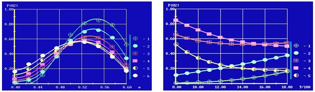
Based on these data, we calculate a number of regression equations for the dependence of PH2[RH2] on m = 0.4–0.6 and T = 800–1800oK, the graphs of which are presented in Fig. 16, 17.
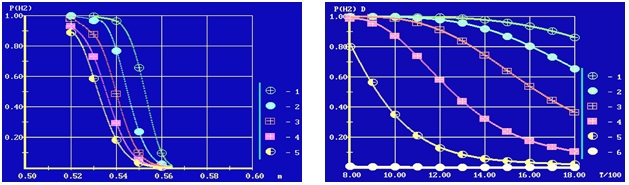
Figure 20. Dependence of the equilibrium pressure of hydrogen PH2 of the direct reduction reaction of iron oxides on the oxidation state of the ore mixture m at different temperatures.
Figure 21. Dependence of the equilibrium pressure of hydrogen PH2 of the direct reduction reaction of iron oxides on temperature at different oxidation states of the ore mixture m.
1 – 800оК; 2 – 1000оК; 3 – 1200оК; m: 1–0.4; 2–0.45; 3–0.5; 4–0.55; 5–0.6
4 – 1400оК; 5 – 1600оК; 6 – 1800оК
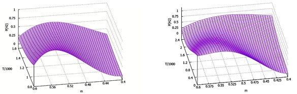
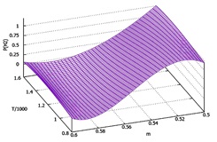
Figure 22. 3D-graph of the dependence of the equilibrium pressure of hydrogen PH2 on the oxidation state of the renewable ore m = 0.4 ÷ 0.6 and on the temperature T = 800 ÷ 1600oK
Figure 23. 3D-graph of the dependence of the equilibrium pressure of hydrogen PH2 on the oxidation state of the renewable ore m = 0.4 ÷ 0.6 and on the temperature T = 0 ÷ 2400oK
Differential equation of the reaction of deoxidation of iron oxides by hydrogen
Suppose that metal oxides (under the action of the reducing agent) remain in the fraction of bound oxygen ∆m, then it will react with the same molar fraction H2. The reaction equation will look like this:
((1-m) + ∆m) Fe1-mOm + ∆m H2 = (1-m) Fe1-m+∆mOm-∆m + ∆m H2O (45)
If we divide the equation by ∆m, then:
((1-m) + ∆m)/∆m Fe1-mOm + H2 = (1-m)/∆m Fe1-m+∆mOm-∆m + H2O (46)
Let's open the expression in parentheses on the left (1-m) + ∆m and divide the components by ∆m. Then we get:
Fe1-mOm + (1-m)/∆m Fe1-mOm + H2 = (1-m)/∆m Fe1-m+∆mOm-∆m + H2O (47)
Let's move the second term on the left (1-m)/∆m Fe1-mOm to the right side of the equation:
Fe1-mOm + H2 = (1-m)/∆m Fe1-m+∆mOm-∆m – (1-m)/∆m Fe1-mOm + H2O (48)
Now let's combine the two expressions on the right as the difference between the two states of the oxide – at the beginning of the reaction and at the end:
Fe1-mOm + H2 = (1-m)/∆m Fe∆mO-∆m + H2O (49)
Now let's assume that ∆m → 0, in fact to a single molecule, then the difference can be differentiated:
Fe1-mOm + H2 = (1-m)(FedmO-dm)/dm + H2O (50)
The Gibbs energy of deoxidation of metal oxide will look like this:
∆rGo[DH2] = ∆ƒGo[H2O] + (1–m)drGo[FedmO–dm]/dm – ∆ƒGo[Fe1-mOm] (51)
where: ∆rGo[DH2] is the Gibbs energy of the deoxidation reaction.
If we compare the differential component of reduction with the analogous differential component of oxidation represented in (13), we can see that they indicate oppositely directed processes, so the magnitude of energy will be the same, but with the opposite sign, i.e.:
drGo[FedmO–dm]/dm = – dƒGo[Fe–dmOdm]/dm (52)
therefore, it can be replaced with a change of sign in equation (48) and written:
∆rGo[DH2] = ∆ƒGo[H2O] – ((1 – m) dƒGo[Fe–dmOdm]/dm + ∆ƒGo[Fe1-mOm]) (53)
We see that the sum in parentheses corresponds to the Gibbs energy in the differential formula for the formation of iron oxides ∆ƒGo[D] (13).
Then you can write:
∆rGo[DH2] = ∆ƒGo[H2O] – ∆ƒGo[D] (54)
∆rGo[DH2] = (A[H2O] – A[dm]) + (B[H2O] – B[dm])T + (C[H2O] – C[dm])T2 + (D[H2O] – D[dm])T3 (55)
We calculate the coefficients of the Gibbs energy equation for the deoxidation of oxides, for which we take the coefficients for the calculation ∆ƒGo[D] (17-20) and the equation for the Gibbs energy of water formation (33).
Finally, we get the coefficients to deduct ∆rGo[DH2]:
AD = -200.7228 + 244.1760m + 1137.8274m2 + 4079.4164m3 – 5257.4530m4 – 6816.2472m5 – 9909.5850m6 + 14258.6400m7 (56)
BD = (41.0743 + 65.2920m – 789.6516m2 – 616.2668m3 – 892.8821m4 + 5931.8920m5 + 306.6470m6 – 3509.2860m7)*10-3 (57)
CD = (-1.6924 + 1.5327m – 10.7202m2 + 134.3579m3 + 66.9143m4 – 236.0968m5 – 833.0653m6 + 789.7218m7)*10-5 (58)
DD = (5.7232 + 3.0904m + 15.1002m2 – 314.5968m3 – 264.6107m4 + 672.5891m5 + 2141.9284m6 – 2035.0818m7)*10-9 (59)
According to the equations obtained, we calculate the coefficients for ∆rGo[DH2] = AD + BDT + CDT2 + DDT3 in the range m = 0 ÷ 0.6. And then, we calculate the value of ∆rGoT[DH2] according to these coefficients.
Figure 24. Temperature dependence of ∆rGo[DH2] at different oxidation values m
1 – (m = 0.1); 2 – (m = 0.2); 3 – (m = 0.3); 4 – (m = 0.4); 5 – (m = 0.5); 6 – (m = 0.6)
Figure 25. Dependence of ∆rGoT[DH2] on the oxidation state of the ore mixture at temperatures T = 0 ÷ 900°K
Figure 26. Dependence of ∆rGoT[DH2] on the oxidation state of the ore mixture at temperatures T = 1200 ÷ 2400°K
1 – (Т = 0оК); 2 – (Т = 298.15оК); 1 – (Т = 1200оК); 2 – (Т = 1500оК); 3 – (Т = 1800оК);
3 – (Т = 600оК); 4 – (Т = 900оК); 4 – (Т = 2100оК); 5 – (Т = 2400оК);
Figure 27. 3D-graph of the dependence of ∆rGo[DH2] on the oxidation state of the renewable ore m = 0.5 ÷ 0.6 and on the temperature T = 800 ÷ 1600oK
Figure 28. 3D-graph of the dependence of ∆rGo[DH2] on the oxidation state of the renewable ore m = 0 ÷ 0.6 and on the temperature T = 0 ÷ 2400oK
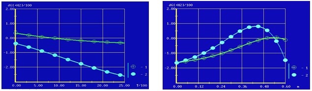
A comparison of the processes of direct reduction of the metal and the gradual deoxidation of the ore mixture of iron oxides is shown in Fig. 29 – 30.
Figure 29. Comparison of ∆rGom(RH2) and ∆rGom(DH2) as a function of T at m = 0.6 (hematite)
Figure 30. Comparison of ∆rGoT(RH2) and ∆rGoT(DH2) depending on m at T = 1200oK
1 – line of values ∆rGom(RH2); 1 – line of values ∆rGoT(RH2);
2 – line of values ∆rGom(DH2); 2 – line of values ∆rGoT(DH2);
From the graph in Fig. 29, it can be seen that direct reduction of hematite is possible only at temperatures above 800°K, deoxidation towards magnetite is more energetically advantageous in all temperature ranges.
From the graph in Fig. 30, it can be seen that deoxidation of hematite at T = 1200°K is energetically more profitable than direct reduction of the metal to m ≥ 0.5378 (between magnetite and wüstite), at lower values of m, direct reduction begins to prevail. It is understood that quantitatively at this point, the total amount of ferrous oxide begins to prevail over the amount of trivalent oxides. If we take a mixture of wüstite and magnesite in a ratio of 1:1, then the arithmetic mean will be m = 0.5425, which is a fairly approximate value to m = 0.5378.
The dependence of the equilibrium hydrogen pressure of the iron deoxidation reaction on the degree of deoxidation of the ore mixture and temperature is shown in Fig. 31-33.
Figure 31. Dependence of the equilibrium pressure of hydrogen PH2 of the iron deoxidation reaction on the oxidation state of the ore mixture m at different temperatures.
Figure 32. Dependence of the equilibrium pressure of hydrogen PH2 of the deoxidation reaction of iron oxides on temperature at different oxidation states of the ore mixture m.
1 – 800oK; 2 – 1000oK; 3 – 1200oK; m: 1 – 0.5; 2 – 0.51361; 3 – 0.525;
4 – 1400oK; 5 – 1600oK 4 – 0.5378; 5 – 0.55; 6 – 0.57143
Figure 33. 3D-graph of the dependence of the equilibrium pressure of hydrogen PH2 of the iron deoxidation reaction on the oxidation state of the ore mixture m = 0.5 ÷ 0.6 and on the temperature T = 800 ÷ 1600oK
References
1. European comission, The European Green Deal, Communication from the Comission: Brussels, 11.12.2019, COM(2019) 640 final. URL: https://eur-lex.europa.eu/legal-content/EN/TXT/?uri=CELEX:52019DC0640 (date of access: 01.26.2025)
2. Adoption of the Paris Agreement, Conference of the Parties, Twenty-first session. Paris: 30 November to 11 December 2015 FCCC/CP/2015/L.9/Rev.1., UNFCCC secretariat. URL: https://unfccc.int/resource/docs/2015/cop21/eng/l09r01.pdf (date of access: 01.26.2025)
3. Stoughton B., Pn.B., B.S. Metallurgy of Iron and Steel, First Edition. USA, NY-UK, London: McGraw-Hill Book Company, 1908. P. 509
4. The hydrogen colour spectrum. Clean Energy Partnership. NationalGrid. 23.02.2023. URL: https://www.nationalgrid.com/stories/energy-explained/hydrogen-colour-spectrum (date of access: 01.22.2025)
5. Atkins P., de Paula J., Keeler J. Atkins’ Physical Chemistry, 11nd Edition. UK, Oxford: University Press, 2018. P. 908
6. Glushko V.P., Gurvich L.V. Termodinamicheskie svoystva individualnih veschestv. Vol. 1, Book 2. 3nd. Moskow: Ed. AN SSSR, Izdatelstvo “Nauka”, 1978. P. 329
7. Iorish V.S., Bergman G.A., Aristova N.M. Termodinamicheskie svoystva individualnih veschestv, Vol. 5, Fe i jego sojedinenija. Moskow: Dep. of Chemistry, St. Univ. URL: https://www.chem.msu.su/rus/tsiv/Fe/welcome.html (date of access: 01.28.2025 (EU))
8. WolframAlpha Program. Computational Knowledge Engine. URL: ttps://www.wolframalpha.com (date of access: 01.26.2025)
9. Program Gnuplot5. URL: https://grafikus.ru/plot3d (date of access: 02.05.2025)
10. Program IrfanWiew. URL: https://www.irfanview.com (date of access: 02.07.2025)
11. Haynes W.M. (ed.). CRC Handbook of Chemistry and Phisics. 95nd ed. London – NY: Boca Raton, FL 33487-2742: CRC Press, Taylor & Francis Group, 2014 – 2015. P. 2665
12. Castellan G.W. Physical Chemistry. Third Edition. US: University of Maryland, Addison-Wesley Publishing Company, 1983. P. 1037
13. Wasserman L. All of Statistics, A Concise Course in Statistical Inference. Berlin, Heidelberg, New York, Barcelona, Hong Kong, London, Milan, Paris, Tokyo: Springer, 2004. P. 459
14. Hastie T., Tibshirani R., Friedman J. The Elements of Statistical Learning, Data Mining, Inference, and Prediction. 2nd Ed. Stanford, California: Springer Series in Statistics, 2017. P. 745
15. Shylov G.E. Matematicheskiy analiz funkcii odnogo peremennogo. part 1,2. M.: Nauka, 1969. P. 528
16. Belanger N. External Fake Constraints Interpolation: the end of Runge phenomenon with high degree polynomials relying on equispaced nodes – Application to aerial robotics motion planning. Camberley, UK: Proceedings - 5th IMA Conference on Mathematics in Defence 23 November 2017. The Royal Military Academy Sandhurst, 2017. P. 9
17. Runge's phenomenon. URL: https://en.wikipedia.org/wiki/Runge’s_phenomenon (date of access: 01.16.2025)
18. Thomas Jr. G.B. et al. Thomas’ Calculus. 13nd Ed. Boston: Pearson Education, 2014. P. 1223
|